
GPON Power Budgets: Sizing Split Ratios Against Real Receiver Sensitivity, Not the Datasheet Ceiling
Sizing a split ratio off the datasheet ceiling looks fine on paper and fails in the field. Here's how to budget against real receiver sensitivity instead.
Pathworks Engineering Team
A GPON optical power budget calculation looks deceptively simple on paper: subtract accumulated losses from OLT launch power, confirm the result clears the ONT's receiver sensitivity threshold, and the design is validated. Most published split-ratio guidance treats the exercise exactly this way: select Class B+ optics, stay under a 1:64 split ratio, and consider the budget closed. The problem with this approach is that "clears receiver sensitivity at time of turn-up" and "designed with adequate margin across the plant's operating life" are two fundamentally different claims, and conflating them is where GPON power budgets fail three or four years into service, not at the point of initial acceptance testing.
This article walks through what the standard GPON budget classes actually guarantee, where real-world as-built budgets systematically diverge from the theoretical calculation, and how to build a split-ratio decision that survives the plant's full operating life rather than just its commissioning test.
The Standard Budget Classes, and What They Actually Guarantee
ITU-T Recommendation G.984.2 defines the standard GPON optical budget classes for the physical media dependent layer: Class B+ at a maximum path loss of 28 dB, and Class C+ at 32 dB, with newer XG-PON and NG-PON2 systems defined under separate ITU-T recommendations extending these budgets further to support higher split ratios and longer reach. That 28 dB or 32 dB figure represents the maximum allowable optical path loss between the OLT and the ONT under the standard: it is a ceiling, not a design target, and treating it as a target rather than a limit is the single most common budget error we encounter when reviewing submitted low-level design packages.
The distinction matters because a design that calculates loss right up to the class ceiling has, by definition, zero margin remaining to absorb anything that happens after the network is accepted and placed into service: no margin for future splice re-entry during maintenance, no margin for connector degradation from repeated mating and unmating cycles, no margin for fiber aging, and no margin for the inevitable difference between as-designed and as-built loss values that shows up on every real construction project regardless of how carefully the design was executed.
Where Real Budgets Diverge From the Class Ceiling
Splitter insertion loss versus theoretical split loss. A 1:32 passive splitter's theoretical loss, calculated from the basic split-ratio formula of 10 × log₁₀(32), works out to approximately 15.05 dB. That theoretical figure is not what a real manufactured component delivers in the field. Manufacturer datasheets for PLC (planar lightwave circuit) splitters typically specify maximum insertion loss in the range of 17.5 to 18.5 dB for a 1:32 device once excess loss inherent to the splitting chip and the connector loss at the splitter housing itself are both included in the specification. Designing a budget against the theoretical 15.05 dB figure instead of the datasheet's actual maximum insertion loss figure routinely erases two to three decibels of assumed margin before a single field splice has even been made: margin that the designer believed existed on paper but that was never actually available.
Two-stage split architectures compound the gap. A common central-office-to-cabinet-to-drop architecture (for example, a 1:4 split at the OLT-adjacent location followed by a 1:8 split at a field cabinet) produces a combined loss that is not simply the arithmetic sum of the two components' theoretical values. Each stage carries its own excess loss beyond the theoretical split calculation, and cascading two real components in series typically loses meaningfully more than the sum of two ideal, lossless splitters would suggest. A designer working from theoretical split-loss tables rather than real cascaded datasheet values will consistently under-budget a two-stage architecture, and the error grows with each additional stage in the split topology.
Connector and splice accumulation over distance. As covered in more depth in our earlier post on fiber splice loss budgets, field fusion splice loss regularly runs above the roughly 0.05 dB figure quoted on splicer manufacturer datasheets once real-world field conditions (dirty fiber ends, minor misalignment, mismatched core geometries between fiber batches from different manufacturing lots) are accounted for honestly. Over a distribution run exceeding twenty kilometers with multiple splice points along its length, this discrepancy alone can consume close to a full decibel of the class budget that a theoretical calculation never anticipated.
Wavelength-dependent attenuation. GPON systems operate downstream at 1490 nm and upstream at 1310 nm, with an optional RF video overlay signal, where present, running at 1550 nm. Fiber attenuation, connector return loss, and splitter performance all vary meaningfully by wavelength. A power budget calculated only at 1310 nm and then applied uniformly across all three wavelengths will systematically understate loss at 1490 nm: which happens to be the wavelength actually carrying the ONT's downstream data-plane signal, meaning the wavelength where the error matters most is exactly the one a 1310 nm-only calculation gets wrong.
Building the Design Margin Correctly
A defensible GPON power budget reserves design margin (commonly two to three decibels) beyond the worst-case as-built calculation, specifically to absorb aging, future splice re-entry for maintenance and augmentation, and connector degradation over a plant life that is typically expected to run fifteen to twenty years or longer. A split-ratio decision made purely against the theoretical class ceiling, without this explicit margin reserve, is a design that will pass initial turn-up acceptance testing and then progressively degrade into service-affecting truck rolls over the following several years, as connectors accumulate mating cycles from routine maintenance activity and splices get re-entered to accommodate new drops or fault repairs.
This margin requirement is also precisely where split-ratio economics and power-budget engineering pull in opposite directions, creating a genuine design trade-off rather than a purely technical calculation. A 1:64 split ratio lowers the cost per home passed by serving more subscribers from a single OLT port, but it consumes budget headroom that a more conservative 1:32 split preserves for the plant's operating life. This trade-off should be quantified on a per-project basis against the specific distance profile and anticipated splice count of the actual route under design: not defaulted to whatever split ratio happened to work on the previous project, since two projects with identical split ratios can have meaningfully different loss profiles depending on distance and splice density alone.
How This Interacts With Splitter Placement Strategy
Splitter placement (centralized at the OLT location versus distributed at field cabinets closer to subscribers) has direct power-budget implications that are frequently overlooked when the placement decision is driven purely by construction cost or cabinet availability. A centralized splitting architecture concentrates all split loss near the OLT, which simplifies the loss budget calculation for each individual subscriber drop but means that fiber count requirements between the OLT and the field are dramatically higher, since every subscriber's individual fiber must be run all the way back before splitting occurs. A distributed architecture reduces backbone fiber count by pushing the split point closer to subscribers, but introduces two-stage split-loss stacking as discussed above, and typically increases the number of field splice points, each of which contributes to the accumulated loss budget in ways that need to be modeled explicitly rather than assumed away.
Have a project like this to scope?
A sketch, a photo, or a rough spreadsheet is enough to start.
Start a ProjectNeither architecture is universally correct. The right answer depends on subscriber density, backbone fiber cost, and the specific loss budget available once realistic (not theoretical) component values are used throughout the calculation.
Why This Connects to Broader Design Quality
A power budget that has been calculated correctly still has to be communicated in a form that a construction crew, a splicing technician, and a future maintenance engineer can all use without reinterpreting the underlying assumptions. A budget calculation buried in a spreadsheet that never makes it into the construction drawing set provides no protection against a splicing crew choosing a route or splice configuration that silently exceeds the designed margin. This is one of the specific gaps we check for as part of validating whether a design package is genuinely build-ready, discussed further in What Makes a Fiber Network Design "Build-Ready"?
Our low-level fiber designs at Pathworks calculate split-stage loss against manufacturer datasheet values rather than theoretical splitting mathematics, and we explicitly flag any route where the calculated as-built loss leaves less than two decibels of margin against the selected optics class: before construction begins, not after a service call reveals the shortfall. See our FTTx & Telecom Networks service page for more on how this is scoped as part of a full design engagement.
Conclusion
The gap between a theoretical GPON power budget and a real, defensible one is rarely a single large error: it is an accumulation of small, individually reasonable-looking assumptions, each of which shaves a fraction of a decibel off the true available margin. Designing against datasheet values rather than textbook formulas, accounting honestly for two-stage split architectures, and reserving explicit margin for the plant's operating life are what separates a network that passes acceptance testing from one that stays reliably in service for the following two decades.
References
- ITU-T G.984.2: Gigabit-capable Passive Optical Networks (GPON): Physical Media Dependent (PMD) Layer Specification
- ITU-T G.987: 10-Gigabit-capable Passive Optical Networks (XG-PON) Systems
- Related reading: Fiber Splice Loss Budgets: How Much Signal Are You Really Losing?
- Related reading: What Makes a Fiber Network Design "Build-Ready"? A Practical Checklist
- Pathworks services: FTTx & Telecom Networks
Related articles
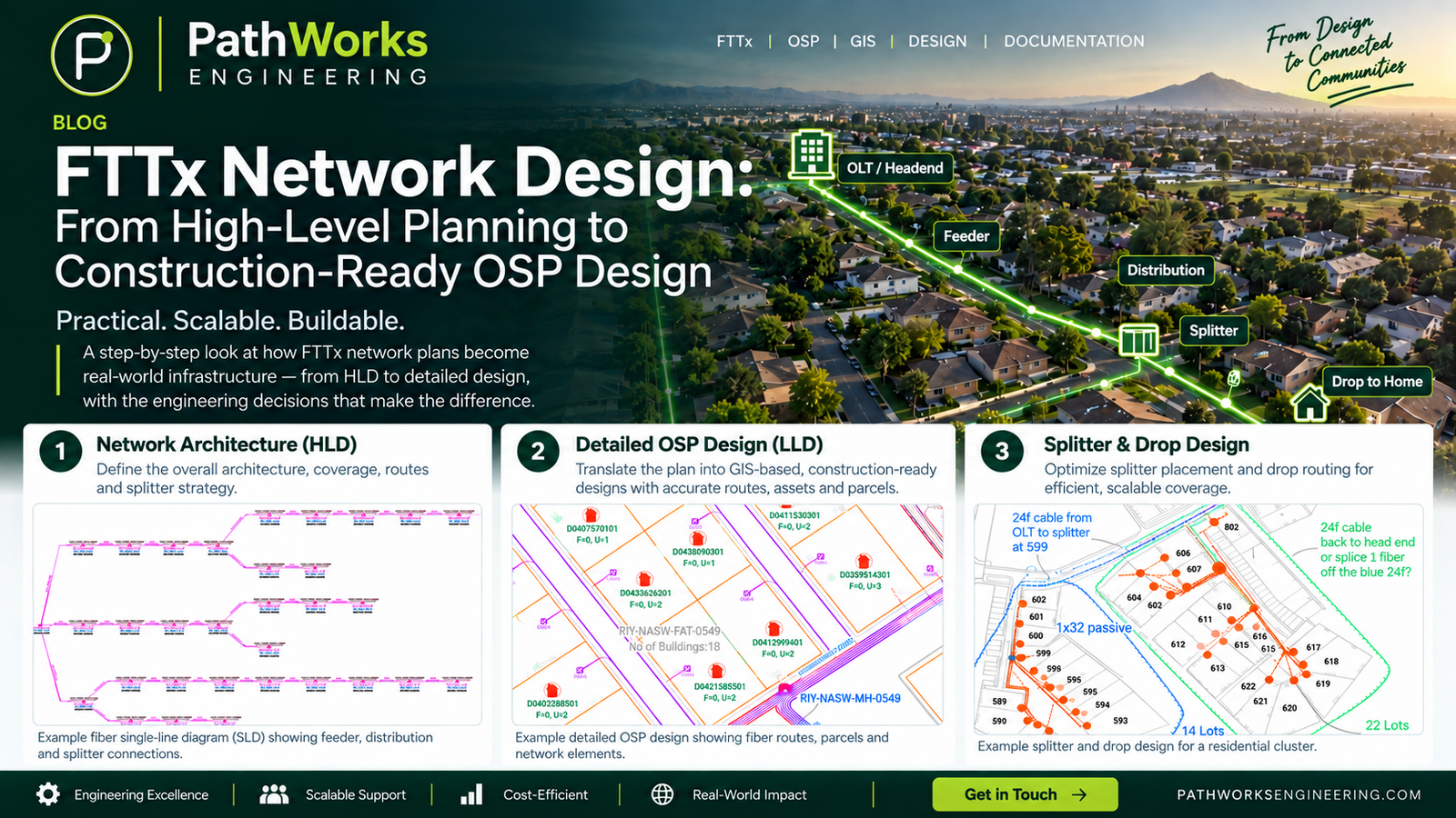

FTTx Network Design: From HLD to Construction-Ready OSP Engineering
A practical guide to FTTx network design, covering HLD, LLD, splitter planning, fiber topology, BOQ development, QA/QC and construction-ready OSP documentation.

As-Built Redlining: Why the Built Network Stops Matching the Design, and How to Control the Drift
The network in the field and the network on the drawing start drifting apart the moment construction begins. Here's how to control that drift instead of discovering it years later.

OSP Route Selection: The Real Cost Model Behind Underground vs. Aerial
A per-foot cost comparison hides most of what actually determines whether an aerial or underground route finishes on schedule and on budget. Here's the data that belongs in the decision instead.